Hello, World!
Let’s get our feet wet! You will now write your first application, and progressively extend its capabilities.
Timeflux apps are written in YAML. If you don’t know anything about YAML, we recommend to first spend three minutes watching this introduction video.
For this app, we will use a node that comes from the timeflux_example plugin. The installation is straightforward:
conda activate timeflux
pip install timeflux_example
For your first iteration, here is what you will build:
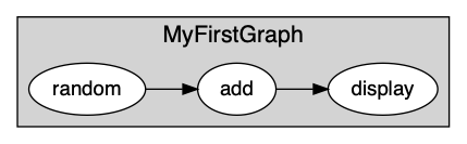
This is a very simple app with one graph and three nodes. The first node generates random time series, sends its output to another node that adds 1 to each value of the matrix, and that itself sends its own output to a debugging node.
Open a code editor, and copy-paste the following:
graphs:
  - id: MyFirstGraph
    nodes:
    - id: random
      module: timeflux.nodes.random
      class: Random
      params:
        columns: 5
        rows_min: 1
        rows_max: 10
        value_min: 0
        value_max: 5
        seed: 1
    - id: add
      module: timeflux_example.nodes.arithmetic
      class: Add
      params:
        value: 1
    - id: display
      module: timeflux.nodes.debug
      class: Display
    edges:
    - source: random
      target: add
    - source: add
      target: display
    rate: 1
Save the file as helloworld.yaml, and run the app (don’t forget to activate the timeflux environment if it is not already the case!):
timeflux -d helloworld.yaml
Interrupt with Ctrl+C.
Let’s take a step back and examine the code. The first thing we notice is the graphs list. Here, we only have one graph. Graphs have four properties:
id– This is not mandatory, but very useful when you have more complex applications. Each time something is logged in the console, the graphidwill be printed, so you know exactly where it comes from.nodes– This is the list of individual computing units in our graph.edges– This is where you connect the nodes together.rate– The frequency of the rate. A value of 25 means that each node in the graph will be executed 25 times per second. The default value is 1, so here, we could have omitted it.
Nodes have also four properties:
id– A unique identifier for the node. Unlike graphids, nodeids are mandatory.module– The name of the Python module where the node is defined.class– The name of the Python class that defines the node.params– A dictionary of parameters passed during the initialization of the node.
The list of parameters and their meaning can be found in the API documentation. In our case:
timeflux_example.nodes.arithmetic.Add()
Edges connect nodes together. They have two properties, source and target. Each of them takes a node id as value. Here we connect the default output to the default input, so we don’t need to specify the port name. We will see how to connect I/O to named and dynamic ports in a moment.
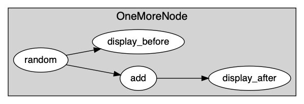
Right now, we have a very simple app that prints the modified matrix in the screen. What if we want to also display the original matrix before we add 1?
This can be represented schematically as:
And in YAML as:
graphs:
  - id: OneMoreNode
    nodes:
    - id: random
      module: timeflux.nodes.random
      class: Random
    - id: add
      module: timeflux_example.nodes.arithmetic
      class: Add
      params:
        value: 1
    - id: display_before
      module: timeflux.nodes.debug
      class: Display
    - id: display_after
      module: timeflux.nodes.debug
      class: Display
    edges:
    - source: random
      target: add
    - source: random
      target: display_before
    - source: add
      target: display_after
We just added one Display node and one edge. For brevity, we also removed the params property of the Random node and used the default values.
All this console printing is boring. We want glitter and unicorns! Or at least, we want to display our signal in a slightly more graphical way. Enters the timeflux_ui plugin. This plugin enables the development of web interfaces, and exposes a JavaScript API to interact with Timeflux instances through WebSockets. Bidirectional streaming and events are supported, as well as stimulus scheduling with sub-millisecond precision. A monitoring interface is included in the package.
Without further ado, let’s install it:
pip install timeflux_ui
We need to refactor our code a little bit. For better performances (and also for readability), it is a good practice to divide the code into multiple graphs. Remember that nodes inside a graph run sequentially and that graphs inside an application run in parallel.
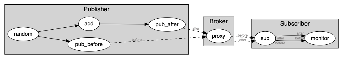
Of course, in our simple example, we could get away with only one graph, but this is an opportunity to introduce a fundamental notion: inter-graph communication. To send and receive information between nodes from different graphs, we can use any of the asynchronous network nodes provided with Timeflux. If you come from the Brain-Computer Interface field, you probably already know about the Lab Streaming Layer system. We have nodes for that (see: timeflux.nodes.lsl). Here we will use a Publish/Subscribe protocol, built on top of the ZeroMQ library, and available in the timeflux.nodes.zmq module. In the Pub/Sub pattern, subscribers express interest in topics, and receive data matching these topics. There can be more than one publisher per topic. Our implementation provides a broker that centralizes messages emitted by publishers.
This will look like this:
It can be rendered in YAML as follows:
graphs:

  - id: Broker
    nodes:
    - id: proxy
      module: timeflux.nodes.zmq
      class: Broker

  - id: Publisher
    nodes:
    - id: random
      module: timeflux.nodes.random
      class: Random
      params:
        columns: 2
        seed: 1
    - id: add
      module: timeflux_example.nodes.arithmetic
      class: Add
      params:
        value: 1
    - id: pub_before
      module: timeflux.nodes.zmq
      class: Pub
      params:
        topic: before
    - id: pub_after
      module: timeflux.nodes.zmq
      class: Pub
      params:
        topic: after
    edges:
    - source: random
      target: add
    - source: random
      target: pub_before
    - source: add
      target: pub_after

  - id: Subscriber
    nodes:
    - id: sub
      module: timeflux.nodes.zmq
      class: Sub
      params:
        topics: [ before, after ]
    - id: monitor
      module: timeflux_ui.nodes.ui
      class: UI
    edges:
      - source: sub:before
        target: monitor:before
      - source: sub:after
        target: monitor:after
What changed:
We added a graph called Broker with only one node. Its role is to centralize the messages. It acts as a proxy between publishers and subscribers.
Our main graph is now called Publisher. We replaced the
Displaynodes byPubnodes. Notice that these nodes take one parameter:topic.A third graph named Subscriber was introduced. The
Subnode subscribes to the two existing topics. TheUInode is responsible for handling the web server and displaying the data. TheSubnode has dynamic output ports, meaning that it will create output ports on the fly, named after thetopicsparameter. TheUIhas dynamic input ports, created automatically according to the second part of thetargetproperty of the edges.sub:beforetomonitor:beforemeans: connect thebeforeoutput port of thesubnode to thebeforeinput port of themonitornode*.
Launch the app, and visit http://localhost:8000/monitor in your browser. From the Streams panel, select one signal, then select the channel you want to display (or choose all channels). Click the Display button, and voilà!
Note
Agreed, this first application does not do anything useful. But by now, you have grasped the essential concepts and are well on your way to a real-world app!